CV? Curriculum Vitae? Oh, Conduction Velocity!

Getting deeper in the calculus of substrate magnitudes

It has been a while since I began the journey of my PhD. I remember that, especially in the first months, I spent a lot of my time reading about atrial fibrillation (AF), therapies to treat it, like pulmonary vein isolation (PVI), techniques to characterise atrial substrate, such as late gadolinium enhancement MRI (LGE-MRI) and magnitudes describing this substrate, including low voltage areas (LVA), image intensity ratio (IIR) or conduction velocity (CV). You can see how many abbreviations we scientists use! It’s easy to get lost. But don’t worry, it has happened to all of us. 

As an example, there is this time I was introducing myself into the description of CV and I was reading a review paper on how to calculate it. I got a call and had to stop reading. When I came back, I read CV and thought the authors were talking about their Curriculum Vitae! It doesn’t happen anymore (well, almost never at least…), but I was seriously confused for a few seconds there. 

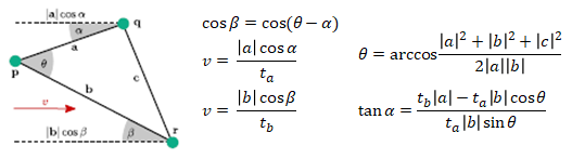
Apart from the confusion I felt then, I also remember the content of the paper from Cantwell et al. It is an interesting review and it also gets deeper in how to obtain information of the CV based on the activation data obtained from endocardial mapping. Hence, in this post I will try to explain two of the methods used to calculate CV from activation data

The first techique I will explain is called “triangulation”. This method usestrigonometry for the calculation of the distance between points captured in the electroanatomical maps. In order to use this method, it is necessary to group the different points of the mesh in triplets and it is assumed that the wavefront crosses the points locally in a planar way. Bearing this in mind it is possible to calculate the CV with different trigonometric equations that relate the speed and the angle of incidence of the wavefront. An illustration of this method and the equations used for the obtention of CV can be seen in Figure 1.

Figure 1: visual concept of triangulation and trigonometric equations to obtain CV [1]

Another option to calculate CV is the “wavefront averaging method”. In this case, the wavefront is also assumed to be locally planar. However, CV is calculated in a more straightforward manner: CV is locally calculated for each point acquired in the electroanatomical map by dividing the linear distance of that point from the reference over the time needed for the wavefront to activate that point. Then, this local CV value is averaged by the 5 local CV values of the 5 neighbouring points. To avoid the inclusion of CV measurements in a different direction than that of activation propagation, points with difference in local activation time of less than 5 ms from the reference point were excluded [2]. A visual representation of this method can be seen in the figure below.

Figure 2: graphic representation of the wavefront averaging method

In the group we are experimenting with these methodologies and hope to get encouraging results in the future. In the meantime, you can read how the other ESRs are doing in their project in our website. Stay tuned for more in the next posts.

See you soon!

Eric


If you want to join me and the rest of the network in our journey, don’t forget to follow us in our social media using the hashtag #PersonalizeAF!